Electric Vehicle Market Size, Share & Forecast, 2021-2028

Electric Vehicle Market Size, Trends, Growth, Report 2022-2030

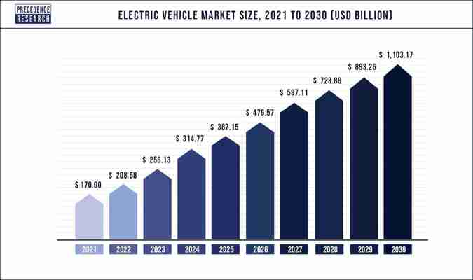
The global electric vehicle market was estimated at USD 170 billion in 2021 and is expected to reach over USD 1103.17 billion by 2030, poised to grow at a compound annual growth rate (CAGR) of 23.1% during the forecast period 2022 to 2030.

Key Takeaway

By 2040, the Europe is expected to achieve 40% greenhouse gas reduction and net-zero by 2050

EV sales increased by 80% in the United States in 2019

Asia Pacific electric vehicle market was valued at USD 121.7 billion in 2021

By propulsion type, the battery electric vehicles (BEV) accounted largest revenue share 66% in 2021

The hybrid electric vehicle segment is expected to reach USD 301.67 billion by 2030 from valued at USD 77,581.7 million in 2021.

The plug-in hybrid EV segment is expected to hit revenue USD 385,617 million from 2022 to 2030.

The passenger car electric vehicle market was valued at USD 127,394 million in 2021 and is projected to hit at USD 598,735 million by 2030.

The commercial vehicle EV market was valued at USD 47,351.9 million in 2021.

The luxury EV market is projecte to reach USD 441,273 million by 2030 from valued at USD 104,380 million in 2021.

The growing funding and investments by key market players drive the electric vehicle market growth. Ford had previously stated that it would invest $11.5 billion in electrifying its vehicle lineup between now and 2022. It recently claimed that it had upped its spending on driverless and electrified vehicles to help boost vehicle sales in the face of ongoing lockdowns. Mercedes-Benz also confirmed that it will release 25 new plug-in hybrid electric vehicles and entirely electric cars by 2025. Companies' diverse product offers have attracted many customers, resulting in an expanding market for electric vehicles.

Growth Factors

A significant number of initiatives taken by the government of various countries, such as tax rebates, subsidies & grants, and other non-financial benefits in car registration and access to carpool lanes expected to drive the sale of electric vehicles in the coming years. For instance, in November 2019, German car manufacturers raised their cash incentives for electric cars to move away from the transition from combustion engines to battery-powered engines to reduce harmful emissions. Countries such as the U.S., China, and different countries in Europe, have registered significant growth in the sale of electric vehicles in the past few decades that, in turn, will contribute to the market growth.

However, lack of charging infrastructure, variations in setting load & lack of standardization are some significant factors hindering the market growth. Different regions, such as China, Europe, the U.S., Japan, Korea, and others, have different standards for electric vehicle charging. Some electric vehicle manufacturers, such as Tesla Inc., are focusing on global standardization of charging infrastructure to overcome this drawback. Nevertheless, the rising adoption of electric vehicles in government and commercial sectors is anticipated to drive the market. For instance, in 2020, the U.K. government approved 200 electric buses with an ambition to make all buses fully electric by 2025, which could save nearly 7,400 tonnes of CO2 every year.

Increase in demand for fuel-effective, high- performance, & low- emigration vehicles

Strict government rules & regulations toward vehicle emigration along with reduction in cost of electric vehicle batteries and adding fuel costs

Lack of high manufacturing cost, charging structure, and range serviceability and anxiety

The market of electric vehicles is likely to be affected positively by the recent trend of self-driving trucks. Furthermore, the top OEMs, similar to Volvo, Daimler Vera, and Tesla, are among others that have been developing automatic-driving electric vehicles for the market. Therefore, technology regarding self-driving will surge the demand for electric cars, in the long run, owing to the colorful advantages of decreased accident threat, easy use, and presence of value-added features. This technology is anticipated to develop in the coming 5-6 times. Therefore, the growth of self-driving electric vehicle technology will likely bring growth opportunities for the market in the forthcoming period.

Market Dynamics

Drivers

Growing government initiatives

Governments are spending a lot on incentives and subsidies to persuade people to buy electric cars. Governments worldwide are taking initiatives likely to boost demand for electric vehicles in the coming decade. Electric vehicles have been regulated in developing countries, and fuel economy criteria have been established in all countries. In addition, they offer incentives and subsidies to electric vehicle makers and buyers. Thus, this factor is driving the market growth.

Restraints

Lack of standardization

The non-presence of standardization among nations may affect charging station connections and hinder market expansion. Using several charging standards worldwide creates a hurdle to harmonizing electric vehicle charging stations. Standardizing charging points would make it easier to set up electric cars in public and contribute to a faster increase in electric vehicle demand worldwide. As a result, the lack of standardization restricts the market's growth.

Opportunities

Declining costs of electric vehicle batteries

Due to technological breakthroughs and the mass production of electric vehicle batteries in huge quantities, the cost of electric vehicle batteries has decreased over the last decade. Because electric vehicle batteries are one of the car's most expensive components, this has reduced the cost of electric vehicles.

Challenges

Lack of charging infrastructure

There are few electric vehicles charging facilities in many places around the world. As a result, public electric vehicle charging stations for electric cars are becoming less available, lowering uptake. Electric vehicle charging infrastructure is being installed in many countries. However, most countries, except a few states, have yet to be able to establish the requisite number of charging stations.

Report Scope of the Electric Vehicle Market

Report Highlights Details Market Size in 2021 USD 170 Billion Growth Rate CAGR of 23.1% from 2022 to 2030 Largest Market Asia Pacific Fastest Growing Market Europe and North America Base Year 2021 Forecast Period 2022 to 2030 Segments Covered Propulsion Type, Components, Vehicle Type, Vehicle Class, Top Speed, Vehicle Drive, EV Charging Point Type, V2G, Region Companies Mentioned BYD Company Ltd., Ford Motor Company , Daimler AG , General Motors Company, Mitsubishi Motor Corporation and Groupe Renault

COVID-19 Impact Analysis:

The COVID-19 pandemic has had an adverse effect over electric vehicle industry.

The registration of all types of electric vehicles during the year 2021 dropped by more than 20%as compared with the number of new EV registrations in the year 2020.

During the pandemic various players are trying to implement different approaches in order to survive the condition by using electric vehicles for product supplies as it provides inexpensive transportation with excellent maneuverability.

Propulsion Type Insights

Battery Electric Vehicles (BEV) led the global market and accounted for more than 66% of the overall revenue share in 2021. The significant growth of the BEV is mainly due to the potential benefits offered, such as control over greenhouse gas (GHG) emissions, energy security concerns, and control over local pollutants. This can be due to people's growing awareness of the environment and the benefits of battery electric vehicles.

Moreover, the cost associated with BEV is more significant compared to the PHEV. The PHEV is expected to witness the fastest CAGR of around 43.5% owing to numerous benefits over BEV; some are low battery cost with smaller battery size and more extended driving range as they are equipped with liquid fuel tanks and internal combustion engines. Additionally, many EV manufacturers such as Volkswagen Group and General Motors are focusing on multi-platform technology with extensive attention towards PHEVs as they can be refueled at any gas station. At the same time, BEVs can only be charged at public charging stations, and public charging spots are far between and very few in the city. Thus, PHEV offers flexibility and freedom to drivers. In January 2020, Volkswagen AG increased its plug-in electric car sales by 60%, from nearly 50,000 to over 80,000 in 2019.

The fuel cell electric vehicles segment is anticipated to grow at the loftiest CAGR during the cast period. This segment's rapid-fire growth is substantially attributed to the adding demand for vehicles with low carbon emigrations, strict carbon emigration morals, and growing emphasis on the relinquishment of FCEVs owing to benefits associated with fast refueling adding government enterprise and investments for advancing fuel cell technology.

Vehicle Type Insights

Based on vehicle type, the electric vehicles market is segmented into heavy commercial vehicles, passenger vehicles, e-scooters & bikes, two-wheelers, and light commercial vehicles. The passenger vehicles segment dominated the electric vehicle market in 2021 with the largest revenue share. This is owing to the governments' substantial backing for electric passenger vehicles in these countries.

The light commercial vehicles segment is anticipated to grow at the loftiest CAGR during the cast period. This segment's rapid-fire growth is substantially attributed to the growing consumer awareness regarding the part of electric vehicles in reducing emigration, the surge in demand for electric cars to reduce line emigrations, and strict government rules and regulations towards vehicle emigration.

End-Use Insights

Based on end use, the electric vehicle market is segmented into private, commercial, and industrial use. The commercial use segment will likely grow at the loftiest CAGR during the forthcoming period. This segment's high growth is credited to the rise in fuel prices and strict emigration morals set by governments, the growing relinquishment of independent delivery vehicles, and the adding relinquishment of electric motorcars and cars.

The rapid expansion of this segment can be attributed to rising fuel prices and government-imposed severe emigration morality, the growing relinquishment of independent delivery vehicles, and the increasing relinquishment of electric motorcars and cars.

Regional Insights

Asia Pacific dominated the global electric vehicle market in 2021 and is expected to be the most lucrative region during the forecast period. China is the primary electric vehicle market globally, accounting for nearly half, 45% of the global electric vehicle sale. Other countries such as Japan, Korea, and India are also opportunistic markets as the governments of these countries are significantly investing in EV startups to promote the manufacturing and sale of EVs across the globe. In July 2019, the Japanese firm Mitsui & Co. invested USD 13.3 million in an Indian e-Vehicle startup, SmartE. The investment would help SmartE to bring multiple synergies in the global EV market for its long-term growth. Similarly, in June 2019, Toyota Motor Corp. invested USD 2 Bn to develop electric vehicles in Indonesia.

The governments of developing and developed nations are providing subsidies to market players, and stringent regulations are driving the growth of the electric vehicle market in the Asia-Pacific region. China's Ministry of Transport provides grants and other incentives for developing low-emission bus fleets, affecting the market even more favorably. Despite the COVID-19 outbreak, Chinese bus manufacturers sold 61,000 additional new energy buses in 2020.

Europe and North America witness substantial growth in the global electric vehicle market. This is attributed to the increasing demand for electric vehicles in the U.S., Norway, France, and Germany. Germany and Norway are the leading markets in the European region, witnessing a CAGR of nearly 40%. Moreover, to promote electric vehicles in North America, policymakers, automotive manufacturers, and charging network companies have launched a non-profit organization called ‘Veloz.’ The organization aimed to attract innovation, investment, marketing, and growth in the electric vehicles market. Electrify America, a U.S.-based electric vehicle manufacturer, announced to invest of USD 2 Bn in Zero Emission Vehicle (ZEV) infrastructure across the U.S. over ten years from 2017 to 2027, out of which USD 800 Mn was invested in California, one of the largest ZEV markets across the world.

The upsurge in the growth of the electric vehicles market in the European region is highly attributed to the harmonious developments in implementing strict emigration regulations by the European Union and adding a focus on reducing the number of conventional buses. Norway leads the way for electric mobility relinquishment in Europe. The share of battery electric vehicles in new auto deals rose to 54.3% in 2020, which is anticipated to surpass 65% of the market share in 2021.

The U.S. is dominating the electric vehicle market in the North American region, and the rising demand for electric automobiles in the U.S. accounts for this proportion. In addition, Electrify America, a non-profit organization dedicated to promoting electric vehicle adoption, announced intentions to invest $200.0 million in California in 2018. As a result, demand for electric vehicles in North America is expected to rise over the projection period.

Key Developments in the Marketplace:

BMW will debut its new i4 electric vehicle in November 2021, with a range of 300-367 miles. In just four seconds, the car can reach 100 km/h. It has an automatic transmission and is equipped with linked car capabilities.

In April 2021, the key player named Toyota introduced the new Mirai & LS models in the city japan which come with the technology of advanced driving assessment.

In April 2021, the key player named BYD introduced four new electric vehicle models which were equipped with Blade batteries in Chongqing. The new vehicle models, Qin plus EV, E2 2021 Tang EV, and Song plus EV came with the advanced feature of battery safety.

In April 2021, the key player named Volkswagen reviled the 7 seater ID.6 X and EV ID.6 Crozz manufactured along with SAIC and FAW in China. Furthermore, these vehicles be sold in China only. Also, it comprises of 2 versions of battery, as 77 kWh & 58 kWh and comes in four powertrain configurations.

Tesla, Inc. declared the acquisition of Maxwell Technologies, Inc. in March 2019. The purchase was made with the goal of improving Tesla's batteries and lowering overall costs in order to obtain a competitive edge in the market.

The Nissan Motor Company has surpassed 180,000 consumers, which is the most significant milestone in the LEAF's launch. The latest vehicle from this business is the Ariya, an electric crossover coupe.

Key Companies & Market Share Insights

The global electric vehicle market is consolidated with high competition owing to the presence of many market players. The existing players are significantly focused on innovation and developing new models and technology to overcome the drawbacks and strengthen their roots in the global market. Some market players also invest in EV startups to boost their regional presence. In December 2019, an electric vehicle startup, Rivian, raised USD 1.3 billion in funds from Inc. and U.S.-based automaker Ford Motor Co.

Furthermore, rising initiatives from governments of several regions towards environmental depletion from CO2 emission have forced automakers to switch towards battery-powered or electric vehicles. Merger, acquisition, partnership, and joint venture are the strategies adopted by the companies to retain their market position. For instance, in March 2019, Alternet Systems, Inc. announced its merger and acquisition pipeline to expand electric vehicle technology innovation and production capacity. Some of the prominent players in the electric vehicle market include:

Ampere Vehicles

Benling India Energy and Technology Pvt Ltd

BMW AG

BYD Company Limited

Chevrolet Motor Company

Daimler AG

Energica Motor Company S.p.A.

Ford Motor Company

General Motors

Hero Electric

Hyundai Motor Company

Karma Automotive

Kia Corporation

Lucid Group, Inc.

Mahindra Electric Mobility Limited

NIO

Nissan Motors Co., Ltd.

Okinawa Autotech Pvt. Ltd.

Rivain

Tata Motors

Tesla Inc.

Toyota Motor Corporation

Volkswagen AG

WM Motor

Xiaopeng Motors

Segments Covered in the Report

This research report estimates revenue growth at global, regional, and country levels and offers an analysis of present industry trends in every sub-segment from 2017 to 2030. This research study analyzes market thoroughly by classifying electric vehicle market report on the basis of different parameters including product and region as follows:

By Propulsion Type

Hybrid Vehicles Pure Hybrid Vehicles Plug-in Hybrid Vehicles

Battery Electric Vehicles

Fuel Cell Electric Vehicles

By Components

Battery Cells & Packs

On-Board Charge

Motor

Reducer

Fuel Stack

Power Control Unit

Battery Management System

Fuel Processor

Power Conditioner

Air Compressor

Humidifier

By Vehicle Type

Passenger Cars

Commercial Vehicles

Two-Wheelers

E-Scooters & Bikes

Light Commercial Vehicles

Others

By Vehicle Class

Mid-priced

Luxury

By Top Speed

Less Than 100 MPH

100 to 125 MPH

More Than 125 MPH

By Vehicle Drive

Front-Wheel Drive

Rear Wheel Drive

All Wheel Drive

By EV Charging Point Type

Normal Charging

Super Charging

By V2G

V2B or V2H

V2G

V2V

V2X

By Geography

The Market for Electric Vehicles: Indirect Network Effects and Policy Design

The market for plug-in electric vehicles (EVs) exhibits indirect network effects due to the interdependence between EV adoption and charging station investment. Through a stylized model, we demonstrate that indirect network effects on both sides of the market lead to feedback loops that could alter the diffusion process of the new technology. Based on quarterly EV sales and charging station deployment in 353 metro areas from 2011 to 2013, our empirical analysis finds indirect network effects on both sides of the market, with those on the EV demand side being stronger. The federal income tax credit of up to $7,500 for EV buyers contributed to about 40% of EV sales during 2011–13, with feedback loops explaining 40% of that increase. A policy of equal-sized spending but subsidizing charging station deployment could have been more than twice as effective in promoting EV adoption.

The electrification of the transportation sector through the diffusion of plug-in electric vehicles (EVs), coupled with cleaner electricity generation, is considered a promising pathway to reduce air pollution from on-road vehicles and to strengthen energy security. The US transportation sector contributes to nearly 30% of US total greenhouse gas emissions, over half of carbon monoxide and nitrogen oxides emissions, and about a quarter of hydrocarbons emissions in recent years. It also accounts for about three-quarters of US petroleum consumption. Different from conventional gasoline vehicles with internal combustion engines, plug-in electric vehicles (EVs) use electricity stored in rechargeable batteries to power the motor, and the electricity comes from external power sources. When operated in all-electric mode, EVs consume no gasoline and produce zero tailpipe emissions. But emissions shift from on-road vehicles to electricity generation, which uses a domestic fuel source. The environmental benefit critically depends on the fuel source of electricity generation.1

Since the introduction of the mass-market models into the United States in late 2010, monthly sales of EVs have increased from 345 in December 2010 to 13,388 in December 2015.2 Despite the rapid growth, the market share of electric cars is still small: the total EV sales only made up 0.82% of the new vehicle market in 2015. In the 2011 State of the Union address, President Obama set up a goal of having 1 million EVs on the road by 2015. Based on the actual market penetration, the goal was met less than halfway.3

As a new technology, EVs face several significant barriers to wider adoption, including the high purchase cost, limited driving range, the lack of charging infrastructure, and long charging time. Although EV owners can charge their vehicles overnight at home, given the limited driving range, consumers may still worry about running out of electricity before reaching their destination. This issue of range anxiety could lead to reluctance to adopt EVs especially when public charging stations are scarce. At the same time, private investors have less incentive to build charging stations if the size of the EV fleet and the market potential are small. The interdependence between the two sides of the market (EVs and charging stations) can be characterized as indirect network effects (or the chicken-and-egg problem): the benefit of adoption/investment on one side of the market increases with the network size of the other side of the market.

The objective of this study is to empirically quantify the importance of indirect network effects on both sides of the EV market and examine their policy implications. This is important for at least two reasons. First, while industry practitioners and policy makers often use the chicken-and-egg metaphor to characterize the challenge faced by this technology, we are not aware of any empirical analysis on this issue. Examining the presence and the magnitude of indirect network effects is important in understanding the development of the EV market. If indirect network effects exist on both sides of the market, feedback loops arise. The feedback loops could exacerbate shocks, whether positive or negative, on either side of the market (e.g., gasoline price changes or government interventions) and alter the diffusion path. Ignoring feedback loops could lead to underestimation of the impacts of policy and nonpolicy shocks in this market.

Second, indirect network effects could have important policy implications. As we describe below, policy makers in the United States and other countries are employing a variety of policies to support the EV market. When promoting consumer adoption of this technology, they can subsidize EV buyers or charging station investors or a combination of the two. Both our theoretical and empirical analyses show that the nature of indirect network effects largely determines the effectiveness of different policies. Therefore, understanding indirect network effects could help develop more effective policies to promote EV adoption.

Taking advantage of a rich data set of quarterly new EV sales by model and detailed information on public charging stations in 353 Metropolitan Statistical Areas (MSAs) from 2011 to 2013, we quantify indirect network effects on both sides of the market by estimating two equations: a demand equation for EVs that quantifies the effect of the availability of public charging stations on EV sales, and a charging station equation that quantifies the effect of the EV stock on the deployment of charging stations. Recognizing the endogeneity issue due to simultaneity in both equations, we employ an instrumental variable strategy to identify indirect network effects. To estimate the network effects of charging stations on EV adoption, we use a Bartik (1991)–style instrument for the endogenous number of electric charging stations, which interacts national charging station deployment shock with local market conditions: number of grocery stores and supermarkets. To estimate the network effects of EV stock on charging station deployment, we use current and historic gasoline prices to instrument for the endogenous cumulative EV sales. Across various specifications, our analysis finds statistically and economically significant indirect network effects on both sides of the market. The estimates from our preferred specifications show that a 10% increase in the number of public charging stations would increase EV sales by about 8%, while a 10% growth in EV stock would lead to a 6% increase in charging station deployment.

With the parameter estimates, we examine the effectiveness of the federal income tax credit program which provides new EV buyers a federal income tax credit of up to $7,500.4 Our simulations show that the $924.2 million subsidy program contributed to 40.4% of the total EV sales during this period. Importantly, our analysis shows that feedback loops resulting from indirect network effects in the market accounted for 40% of that sales increase, a significant portion. Our simulations further show that if the $924.2 million tax incentives were used to build charging stations instead of subsidizing EV purchase, the increase in EV sales would have been twice as large. The better cost effectiveness of the subsidy on charging stations relative to the income tax credit for EV buyers is due to (1) strong indirect network effects on EV demand and (2) low price sensitivity of early adopters.

This study directly contributes to the following three strands of literature. First, our study adds to the emerging literature on consumer demand for electric vehicles. The Congressional Budget Office (CBO 2012) estimates the effect of income tax credits for EV buyers based on previous research on the effects of similar tax credits on traditional hybrid vehicles and finds that the tax credit could contribute to nearly 30% of future EV sales. DeShazo, Sheldon, and Carson (2014) use a statewide survey of new car buyers in California to estimate price elasticities and willingness to pay for different vehicles and then simulate the effect of different rebate designs. They estimate that the current rebate policy in California that offers all income classes the same rebate of $2,500 for battery electric vehicles (BEVs) and $1,500 for plug-in hybrid vehicles (PHEVs) leads to a 7% increase in EV sales. Using market-level sales data, our study offers a first analysis to quantify the role of indirect network effects in the market and their implications on government subsidies.

Second, our study fits into the rich literature on indirect network effects. Previous work on indirect network effects dates back to early theoretical studies such as Rohlfs (1974), Farrell and Saloner (1985), and Katz and Shapiro (1985). Our paper is also related to the emerging literature on two-sided markets that exhibit indirect network effects.5 Theoretical work includes Caillaud and Jullien (2003), Armstrong (2006), Hagiu (2006), Rochet and Tirole (2006), and Weyl (2010), and empirical work includes the PDA and compatible software market by Nair, Chintagunta, and Dube (2004), the market of CD titles and CD players by Gandal, Kende, and Rob (2000), the Yellow Pages industry by Rysman (2004), and the video game industry by Clements and Ohashi (2005), Corts and Lederman (2009), Lee (2013), and Zhou (2014). In this strand of literature, our study is closest to Corts (2010) in topic which extends the literature to the automobile market and studies the effect of the installed base of flexible-fuel vehicles (FFV) on the deployment of E85 fueling stations. Corts (2010) only focuses on indirect network effects on one side of the market and does not look at that the effect of E85 fueling stations on FFV adoption.

Third, our analysis contributes to the rich literature on the diffusion of vehicles with advance fuel technologies (e.g., hybrid vehicles) and alternative fuels (e.g., FFVs). Kahn (2007), Kahn and Vaughn (2009), and Sexton and Sexton (2014) examine the role of consumer environmental awareness and signaling in the market for traditional hybrid vehicles. Heutel and Muehlegger (2012) study the effect of consumer learning in hybrid vehicle adoption, focusing on the different diffusion paths of Honda Insight and Toyota Prius. Several recent studies have examined the impacts of government programs both at the federal and state levels in promoting the adoption of hybrid vehicles, including Beresteanu and Li (2011), Gallagher and Muehlegger (2011), and Sallee (2011). Both hybrid vehicles and EVs represent important steps in fuel economy technology. Environmental preference, consumer learning, and government policies are likely to be all relevant in the EV market. Our paper focuses on the key difference between these two technologies: indirect network effects in the EV market. Huse (2014) examines the impact of government subsidy in Sweden on consumer adoption of FFVs and the environmental impacts when consumers subsequently choose to use gasoline instead of ethanol due to low gasoline prices. Based on naturalistic driving data, Langer and McRae (2014) show that a larger network of E85 fueling stations would reduce the time cost of fueling and hence increase the adoption of FFVs.

Section 1 briefly describes the industry and policy background of the study and the data. Section 2 presents a simple model of indirect network effects and uses simulations to show how feedback loops amplify shocks. Section 3 lays out the empirical model. Section 4 presents the estimation results. In section 5, we present the policy simulations and compare the existing income tax credit policy with an alternative policy. Section 6 concludes.

1. Industry and Policy Background and Data In this section, we first present industry background, focusing on important barriers to EV adoption and then discuss current government policies. Next we present the data used in the empirical analysis. 1.1. Industry Background Tesla Motors played a significant role in the comeback of electric vehicles by introducing Tesla Roadster, an all-electric sports car, in 2006 and beginning general production in March 2008. However, the model had a price tag of over $120,000, out of the price range for average buyers. Nissan Leaf ($33,000) and Chevrolet Volt ($41,000) were introduced into the US market in December 2010, marking the beginning of the mass market for EVs. There are currently two types of EVs: battery electric vehicles (BEVs) which run exclusively on high-capacity batteries (e.g., Nissan Leaf), and plug-in hybrid vehicles (PHEVs) which use batteries to power an electric motor and use another fuel (gasoline) to power a combustion engine (e.g., Chevrolet Volt). As depicted in figure 1, quarterly EV sales increased from less than 2,000 in the first quarter of 2011 to nearly 30,000 in the last quarter of 2013, while the number of public charging stations has increased from about 800 to over 6,000. Nevertheless, the EV market is still very small: EV sales only made up 0.82% (or 113,889) of the total new vehicle sales in the United States in 2015, and there are only about 12,500 public charging stations as of March 2016, compared to over 120,000 gasoline stations. Figure 1. National quarterly EV sales and public charging stations. The quarterly EV sales plotted include both BEV and PHEV sales. Source: Authors’ calculations using monthly sales dashboard data and electric charging station location data by Alternative Fuel Data Center of the Department of Energy. There are several commonly cited barriers to EV adoption. First, EVs are more expensive than their conventional gasoline vehicle counterparts. The manufacturer’s suggested retail prices (MSRP) for the 2015 model of Nissan Leaf and Chevrolet Volt are $29,010 and $34,345, respectively, while the average price for a comparable conventional vehicle (e.g., Nissan Sentra, Chevrolet Cruze, Ford Focus, and Honda Civic) is between $16,000 and $18,000. A major reason behind the cost differential is the cost of the battery. As battery technology improves, the cost should come down. In addition, lower operating costs of EVs can significantly offset the high initial purchase costs.6 A recent study by EPRI (2013) compares the lifetime costs (including purchase cost less incentives, maintenance, and operation) of vehicles of different fuel types and finds that under reasonable assumptions, higher capital costs are well balanced by savings in operation costs: EVs are typically within 10% of comparable hybrid and conventional gasoline vehicles. The second notable barrier to EV adoption is the limited driving range. BEVs have a shorter range per charge than conventional vehicles have per tank of gas, contributing to consumer anxiety of running out of electricity before reaching a charging station. Nissan Leaf, the most popular BEV in the United States, has an EPA-rated range of 84 miles on a fully charged battery in 2015. Chevrolet Volt has an all-electric range of 38 miles, beyond which it will operate under gasoline mode. This range is sufficient for daily household vehicle trips but may not be enough for longer distance travels. The third barrier, closely related to the second, is the lack of charging infrastructure. A large network of charging stations can reduce range anxiety and allow PHEVs to operate more under the all-electric mode to save gasoline.7 There are two types of public charging stations: 240 volt AC charging (level 2 charging) and 500 volt DC high-current charging (DC fast charging), with the former being the dominant type. The installation of charging stations involves a variety of costs, including charging station hardware, other materials, labor, and permits. A typical level 2 charging station for public use has three to four charging units and costs about $27,000, while a DC fast charging station costs over $50,000.8 Charging stations can be found at workplace parking lots, shopping centers, grocery stores, restaurants, dealers, and existing gasoline stations, a point that we will come back to when constructing the instrument for the number of charging stations in the EV demand estimation. Owners of charging stations are often motivated by a variety of considerations such as boosting their sustainability credentials, attracting customers for their main business, and providing a service for employees. Charging stations are often managed by one of the major national operators such as Blink, ChargePoint, and eVgo. The fourth barrier is the long charging time. It takes much longer to charge EVs than to fill up gasoline vehicles. A BEV may not be able to get fully charged overnight if just using a regular 120 volt electric plug (e.g., it takes 21 hours for a Nissan Leaf to get fully charged). To get faster charging, BEV drivers either need to install a charging station at home or go to public charging stations. It takes six to eight hours to fully charge a Nissan Leaf at a level 2 charging station and only 10–30 minutes at a DC fast charging station.9 Unlike BEVs, PHEV batteries can be charged not only by an outside electric power source, but by the internal combustion engine as well. Having the second source of power may alleviate range anxiety, but the shorter electric range limits the fuel cost savings from EVs. 1.2. Government Policy The diffusion of electric vehicles together with a clean electricity grid can be an effective combination in reducing local air pollution, greenhouse gas emissions, and oil dependency. The EV technology is widely considered as representing the future of passenger vehicles. The International Energy Agency projects that by 2050, EVs have the potential to account for 50% of light duty vehicle sales.10 Many countries around the world have developed goals to develop the EV market and provide support to promote the diffusion of this technology (Mock and Zhang 2014).11 To reduce the price gap between EVs and their gasoline counterparts, the Energy Improvement and Extension Act of 2008, and later the American Clean Energy and Security Act of 2009, grant a federal income tax credit for new qualified EVs. The minimum credit is $2,500 and the credit may be up to $7,500, based on each vehicle’s battery capacity and the gross vehicle weight rating. Moreover, several states have established additional state-level incentives to further promote EV adoption such as tax exemptions and rebates for EVs and nonmonetary incentives such as high occupancy vehicle (HOV) lane access, toll reduction, and free parking. California, through the Clean Vehicle Rebate Project, offers a $2,500 rebate to BEV buyers and a $1,500 rebate to PHEV buyers. In addition, federal, state, and local governments provide funding to support charging station deployment. For example, the Department of Energy provided ECOtality Inc. a $115 million grant to build residential and public charging stations in 22 US cities in collaboration with local project partners. Government intervention in this market could be justified from the following perspectives. First, indirect network effects in the EV market represent a source of market failure since marginal consumers/investors only consider the private benefit in their decision, and the network size on both sides is less than optimal (Liebowitz and Margolis 1995; Church, Gandal, and Krause 2002). In addition, given the nature of the market, each side of the market is unlikely to internalize the external effect on the other side through market transactions. If EVs are produced by one automaker, the automaker would have an incentive to offer a charging station network to increase EV adoption. Nissan and GM are the two early producers of EVs, but more and more auto makers are entering the competition. Nissan is a large owner of charging stations but GM is not.12 Second, the external costs from gasoline consumption in the United States and many countries around the world are not properly reflected by the gasoline tax (Parry and Small 2005; Parry et al. 2014). Compared to conventional gasoline vehicles, EVs offer environmental benefits when the electricity comes from clean generation such as renewables. In regions that depend heavily on coal or oil for electricity generation, EVs may not demonstrate an environmental advantage over gasoline vehicles.13 Electricity generation continues to become cleaner around the world due to the adoption of abatement technologies (e.g., scrubbers), the deployment of renewable generation, and the switch from coal to natural gas. In addition, technologies are being developed to integrate EVs and renewable electricity generation such as solar and wind. The integration of the intermittent energy source with EV charging not only can help EVs fully realize its environmental benefits but also can leverage EV batteries as a storage facility to address the issue of intermittency and serve as an energy buffer (Lund and Kempton 2008). Third, technology spillovers among firms often exist, especially in the early stage of new technology diffusion (Stoneman and Diederen 1994). The development of EV technology requires significant costs, but the technology know-how once developed can spread through many channels, including worker migration and the product market. Bloom, Schankerman, and van Reenen (2013) estimate that the social returns to R&D are larger than the private returns due to positive technology spillovers, implying underinvestment in R&D. In addition, the social returns to R&D by larger firms are larger due to stronger spillovers. 1.3. Data We construct a panel data set consisting of quarterly EV sales by vehicle model and the number of charging stations available at 353 MSAs from 2011 to 2013. Table 1 presents summary statistics of the variables used in our regression analysis. Data on quarterly vehicle sales of each EV model in each MSA are purchased from IHS Automotive. The sales data include 17 EV models: 10 BEVs and 7 PHEVs. Due to different introduction schedules, there were two vehicle models in our 2011 data: Nissan Leaf and Chevrolet Volt. The 2012 data include four more vehicle models: Ford Focus EV, Mitsubishi i-MiEV, Fisker Karma, and Toyota Prius Plug-in. The 2013 data include 11 additional models: Honda Accord Plug-in, Ford C-Max Energi, Cadillac ELR, Honda Fit EV, Fiat 500E, Smart ForTwo Electric Drive, Tesla Model S, Porsche Panamera, Toyota RAV4, Chevrolet Spark EV, and Ford Transit Connect EV. In 2013, the top four EV models are Nissan Leaf, Chevrolet Volt, Tesla Model S, and Toyota Prius plug-in with market shares (sales) of 25.8% (22,610), 24.4% (23,094), 17.4% (18,650), and 9.4% (12,088), respectively. Table 1. Summary Statistics Variable Mean SD A. Vehicle demand equation: Sales of an EV model 9.62 40.01 Gasoline prices ($) 3.52 .26 EV retail price − tax incentives ($) 33,161 18,569 No. of charging stations 22.13 45.74 Residential charging stations from the EV project 9.21 65.41 Annual personal income ($) 41,607 82,536 Hybrid vehicle sales in 2007 945 1,859 No. of grocery stores 278 624 Average commute (minutes) 22.96 3.37 College graduate share .40 .07 Use public transport to work share .02 .03 Drive-to-work share .88 .05 Share of white residents .78 .11 No. of observations 14,563 B. Charging station equation: No. of charging stations 9.94 28.13 No. of EV installed base 134 584 Charging station tax credit (%) 4.56 14.7 Public funding or grants .33 .47 No. of grocery stores 186 455 Hybrid vehicle sales in 2007 568 1,354 Current gasoline prices ($) 3.49 .27 Gasoline price last year ($) 3.25 .39 Gasoline price two years ago ($) 2.78 .59 Gasoline price three years ago ($) 2.78 .58 State EV incentives (rebates + tax credits) ($) 1,575 3,121 No. of observations 4,236 For our analysis, we focus on the 353 MSAs (out of 381 MSAs in total) for which observations are available in all three years, and their EV sales accounted for 83% of the national EV sales during our data period. Panel A of figure 2 depicts the spatial pattern of EV ownership (the number of EVs per million people) in the last quarter of 2013. It shows that large urban areas have a higher concentration of EVs. The MSA with the highest concentration is San Jose–Sunnyvale–Santa Clara, CA, with 5,608 EVs per million people by the end of 2013. The next two MSAs are both nearby: San Francisco–Oakland–Fremont and Santa Cruz–Watsonville. The MSA with the lowest concentration is Laredo, TX, with only 36 EVs per million people (nine EVs with a population of a quarter of a million). Figure 2. Spatial distribution of EVs and public charging stations. A, Installed base of EVs per million people. B, Public charging stations per million people. Map boundaries define metropolitan statistical areas. Both graphs are shown for the fourth quarter of 2013. We obtain detailed information on locations and open dates of all charging stations from the Alternative Fuel Data Center (AFDC) of the Department of Energy. By matching the ZIP code of each charging station to an MSA and using the station open date, we construct the total number of public charging stations available in each quarter for each MSA. Panel B of figure 2 shows the spatial distribution of charging stations (the number of charging stations per million people). The pattern is very similar to what we observe in panel A for EV ownership. The correlation coefficient between the two variables is 0.63, partly reflecting the interdependence of EVs and charging stations. The top three MSAs with the most charging stations per million people are Corvallis, OR, Olympia, VA, and Napa, CA, with 210, 170, and 117 public charging stations per million people, respectively. These three MSAs are the number eleventh, fifth, and sixth in terms of the EV concentration in panel A. We collect data on state-level incentives such as tax credits and rebates for both electric vehicles and charging stations from AFDC. From the American Chamber of Commerce cost-of-living index database, we collect quarterly gasoline prices for each MSA from 2008 to 2013. Household demographics are collected from the American Community Survey.

2. A Model of Indirect Network Effects In this section, we use a stylized model to illustrate indirect network effects on both sides of the market (EV demand and charging station investment) and to show how indirect network effects give rise to feedback loops. We then conduct simulations to shed light on how the effectiveness of different types of policies (e.g., subsidizing EV purchases versus charging station investment) hinges on the relative magnitude of indirect network effects on the two sides as well as consumer price sensitivity. The results from the simulations provide a theoretical basis for our empirical findings based on real-world data. 2.1. Model Setup and Properties We assume that EV sales q t (N t , p t , x t ) depends on the number of public charging stations in the market (N t ), the price of the EV (p t ), and other product characteristics combined (x t ) that affect consumers’ choice, such as the fuel cost.14 The installed base of EVs is the cumulative sum of EV sales minus scrappage by the time t, denoted by Q t = ∑ h = 1 t q h * s t , h , where s t , h is the survival rate at time t for EVs sold in time h. The number of charging stations that have been built N t (Q t , z t ) depends on the EV market size Q t and other variables combined z t that might affect the fixed cost of investment. To facilitate the illustration, we specify the following functions for EV demand and charging station deployment: (1) ln ( q t ) = β 1 ln ( N t ) + β 2 ln ( p t ) + β 3 x t , (2) ln ( N t ) = γ 1 ln ( Q t ) + γ 2 z t . The EV demand equation arises from a discrete choice model of vehicle demand and follows closely the logit model using the market-level data as in Berry ( The EV demand equation arises from a discrete choice model of vehicle demand and follows closely the logit model using the market-level data as in Berry ( 1994 ). The charging station equation can be derived from an entry model as in Gandal et al. ( 2000 ), and we derive an empirical counterpart to this equation for our specific context in the appendix. The parameters β 1 and γ 1 capture the magnitude of the indirect network effects on the two sides. Feedback loops (or two-way feedback) arise if both β 1 and γ 1 are nonzero. Intuitively, a shock to the system, for example, an increase in x t , would change EV sales q t , which would in turn affect the installed base Q t plus; 1 . This would then lead to changes in the number of charging stations N t + 1 and hence affect q t + 1 . The impact would circle back and forth between these two equations. If both β 1 and γ 1 are positive, positive feedback loops would arise, and they can amplify the shocks (either positive or negative) in either side of the market, such as a tax credit for EV purchases or subsidy on charging station investment. The parameter β 2 (negative) is the price elasticity of demand and captures consumer price sensitivity. To understand the property of the system such as the existence of the steady state and its property, we assume that the survival rate s t , h is δt − h, where δ < 1. Further assume p t = p , x t = x, and z t = z. Substituting equation (2) into equation (1), we have: (3) ln ( q t ) − β 1 γ 1 ln ( q t + δ Q t − 1 ) = β 1 γ 2 z + β 2 ln ( p ) + β 3 x . The right-hand side β 1 γ 2 z + β 2 ln ( p ) + β 3 x is constant with respect to q t , and we denote it by c. During period 1, Q t − 1 = 0. Solving the equation, we obtain q 1 = exp ⁡ [ c / ( 1 − β 1 γ 1 ) ] . To solve for the steady state solution (q*, N*), we use the steady state condition q t = q t + 1 = q * and find: q * = exp ( c − β 1 γ 1 ln ( 1 − δ ) 1 − β 1 γ 1 ) = q 1 * exp ( − β 1 γ 1 ln ( 1 − δ ) 1 − β 1 γ 1 ) . N * = exp [ γ 1 c − β 1 γ 1 ln ( 1 − δ ) 1 − β 1 γ 1 − γ 1 ln ( 1 − δ ) + γ 2 z ] . The stock of EVs in the steady state Q * = q * / ( 1 − δ ) where the outflow of EVs due to scrappage is equal to the inflow from new EV sales.15 To examine the stability of the steady state, we write Q t − 1 = q t − 1 + δ Q t − 2 and substitute it into equation (3): ln ( q t ) − β 1 γ 1 l n ( q t + δ q t − 1 + δ 2 Q t − 2 ) = c . This defines an implicit function of q t = G ( q t − 1 ) . When β 1 γ 1 < 1 , it can be shown that G ( 0 ) > 0 , G ′ ( ) > 0 , and G ″ ( ) < 0 . Therefore, the steady state solution is stable as shown in figure 3. In our following policy analysis, we take β 1 γ 1 < 1 , which is also confirmed in our empirical analysis. Figure 3. Steady state solution and stability. The expression q t is the number of new EV sales in each period; q t = G(q t − 1 ) is the implicit function defined in equation (3); q * is the steady state solution. The partial effect of vehicle price p on EV sales in the steady state is: ∂ q * ∂ p = exp ( c − β 1 γ 1 ln ( 1 − δ ) 1 − β 1 γ 1 ) β 2 1 − β 1 γ 1 , where β 2 < 0 . When β 1 γ 1 < 1 , this partial effect is negative as economic theory would suggest. Similarly, the changes in other demand side factors captured by x and the changes in the factors in the charging station equation z will both shift G ( q t − 1 ) in where. When, this partial effect is negative as economic theory would suggest. Similarly, the changes in other demand side factors captured byand the changes in the factors in the charging station equationwill both shiftin figure 3 up or down and hence affect the steady state solution of EV sales. 2.2. Implications on Policy Choices Now we conduct simulations to understand how feedback loops magnify policy shocks and their implications on policy choices. We fix p t , x t , and z t in equations (1) and (2) and assume certain values for model parameters as reported in Table 2. We then solve for q t , Q t , and N t sequentially for each period. Because of the positive feedback loops (by assuming both β 1 and γ 1 being positive), EV sales and the number of charging stations will keep growing naturally until they reach the steady state where the inflow of new vehicles equals the outflow of vehicles due to scrappage. To examine how positive feedback loops could amplify a policy shock, we simulate a scenario where all EV buyers are provided with a $7,500 subsidy for the first five periods and no more subsidy is offered afterward. Table 2. Parameters for Simulating Indirect Network Effects Coefficients Values Variables Values β 1 .8 p 30,000 β 2 −1.5 X 16 β 3 1 Z 2 γ 1 .4 γ 2 1 δ .9 As shown in panel A in figure 4, due to both the price effect (captured by β 2 ) and the indirect network effects (captured by β 1 and γ 1 ), the subsidy increases EV sales substantially compared with the no-policy case during the first five periods. When the subsidy terminates, EV sales continue to increase through feedback loops but with a smaller magnitude. The sales increase due to subsidy gets smaller as feedback loops diminish and the two growth paths eventually overlap. In both cases, the path of EV sales converges to the same steady state but the policy shock makes the system converge to the steady state more quickly: indirect network effects expedite this process through positive feedback loops. Figure 4. Impacts of income tax credits (five periods) under feedback loops. A, EV sales increase due to feedback loops. B, Charging stations increase due to feedback loops. EV sales and charging stations without subsidy are solutions given by the system defined in section 3. The simulated subsidy effects are due to a policy design that gives EV buyers a tax credit of $7,500 for the first five periods. The parameters for simulations are reported in Table 2, and the intuitive findings remain with different assumptions of the simulation parameters. Figure 4, panel B, depicts a similar pattern in the dynamic path of charging station deployment. With the positive policy shock on the EV purchase side, the stock of charging stations increases quickly for the first five periods and continues to grow at a decreasing rate after the policy. It eventually converges to the same steady state as in the no-policy scenario. These two graphs demonstrate that feedback loops from indirect network effects magnify a shock to any side of the system and alter the convergence process on both sides. The existence of indirect network effects on both sides of the market could have important policy implications. To foster the development of the EV market, policy makers can choose to subsidize consumers for EV purchase directly (policy 1) or to subsidize charging station investment (policy 2). We conduct simulations to examine the relative cost effectiveness of these two policy options. Policy 1 provides EV buyers with a subsidy of $7,500 per EV in the first five periods. Policy 2 uses the same account of total funding as in policy 1 to build charging stations. We compare the cumulative sales increase over time due to these two policies (with a 5% annual discount rate).16 To examine the implication of the relative strength of indirect network effects on policy choices, we vary the ratio of β 1 /γ 1 by holding β 1 constant while changing γ 1 . Figure 5 depicts, for any given price sensitivity β 2 (say −1.5), as β 1 /γ 1 increases indirect network effects in EV demand become relatively stronger), the second policy (subsidy on charging stations) becomes more and more effective measured by the increase in cumulative sales over time. The two policies are equivalent when β 1 /γ 1 is 1 given the price elasticity of −1.5. Figure 5. Policy comparison and relative strength of indirect network effects. This figure depicts the relationship between the relative policy effects of two subsidy designs and the relative strength of the indirect network effects on both sides of the EV market. Policy 1 subsidizes the EV purchase by tax credits and policy 2 uses the same amount of funding to subsidize charging stations. Given a price elasticity of EVs, policy 2 becomes more and more effective than policy 1 when the effect of charging stations on EV demand (denoted by β 1 ) becomes larger relative to the effect of EV stock on charging stations (denoted by γ 1 ). When the magnitude of the price elasticity increases (decreases) and consumers are more (less) sensitive to prices, policy 2 becomes less (more) effective relative to policy 1 for a given ratio of β 1 /γ 1 . In addition to the relative strength of indirect network effects on both sides, the policy comparison also depends on the price elasticity of EV demand. When consumers are more sensitive to prices (e.g., going from −1.5 to −1.6), the policy of subsidizing charging stations becomes relatively less effective for a given β 1 /γ 1 . This finding is illustrated by the outward shift of the curve when the price elasticity changes to −1.4 and −1.6. The result is intuitive: if consumers are less price sensitive, it would take a larger subsidy on EV purchases in order to push consumers to buy EVs, hindering the effectiveness of the policy. To summarize, the policy of subsidizing charging stations becomes more effective relative to the policy of subsiding EV purchases when indirect network effects on EV demand become stronger (holding network effects on the charging station side constant) or when consumers are less sensitive to price. These findings offer a theoretical foundation for the policy comparison after our empirical analysis.

3. Empirical Framework To investigate indirect network effects on both sides of the market, we estimate: (1) an EV demand equation that examines the effect of charging stations on EV sales and (2) a charging station equation that estimates the effect of athe EV fleet on charging station deployment. These equations build upon equations (1) and (2) in the theoretical model above. 3.1. EV Demand To describe the empirical demand model of EVs, let k index an EV model such as Nissan Leaf and Chevrolet Volt, m index a market (MSA), and t index a year-quarter. We estimate the following equation: (4) ln ( q k m t ) = β 0 + β 1 ln ( N m t ) + β 2 ′ X k m t + T t + δ k m + ε k m t , where q kmt is the sales of EV model k in market m and year-quarter t.N mt denotes the total number of public charging stations that have been built in the MSA by the end of a given quarter.N mt ) captures the effect of charging stations on electric vehicle purchases and the log form allows the effect to be diminishing. The term X kmt is a vector of related covariates including the effective purchase price, personal income, and other control variables. The effective purchase price of a model is defined as the manufacturer’s suggested retail price (MSRP) less the related subsidies (tax credits and tax rebates at both federal and state levels). whereis the sales of EV modelin marketand year-quarter 17 The termdenotes the total number of public charging stations that have been built in the MSA by the end of a given quarter. 18 We use the number of charging stations instead of the total number of charging outlets to represent the availability of charging infrastructure, but the qualitative findings remain if we use the number of charging units. The expression ln() captures the effect of charging stations on electric vehicle purchases and the log form allows the effect to be diminishing. The termis a vector of related covariates including the effective purchase price, personal income, and other control variables. The effective purchase price of a model is defined as the manufacturer’s suggested retail price (MSRP) less the related subsidies (tax credits and tax rebates at both federal and state levels). We also include a full set of year-quarter (e.g., the first quarter of 2011) fixed effects and MSA model (e.g., Nissan Leaf in San Francisco) fixed effects in equation (4). Year-quarter fixed effects T t control for national demand shock for EVs common across MSAs such as consumer awareness. MSA-model fixed effects δ km not only control for time-invariant product attributes such as quality and brand loyalty that could affect vehicle demand but also control for time-invariant local preference for green products (Kahn 2007; Kahn and Vaughn 2009) and demand shocks for each model (e.g., a stronger preference or dealer presence for Nissan Leaf in San Francisco). The term ε kmt is the unobserved demand shocks that are time varying and market specific (for example, unobserved local government subsidy for purchasing EVs or market-specific promotions for a vehicle model that vary over time). It is well documented in the vehicle demand literature that failing to control for unobserved product attributes could lead to downward bias in the price coefficient estimates (for example, Berry, Levinsohn, and Pakes 1995; Beresteanu and Li 2011). MSA-model fixed effects absorbs both observed and unobserved vehicle attributes variations that are time invariant, and what is left is the variation of vehicle attributes over time. Since most of the EV models in our sample appear for only one year and there is little variation of the observed attributes for the models that appear for more than one year, we believe that using MSA-model fixed effects could control for unobserved product attributes and alleviate the need to use the methodology developed in Berry et al. (1995) to deal with price endogeneity where they only have national-level sales data one market).19 The price coefficient is identified from the fact that effective EV prices vary across markets and over time due to state-level subsidies and temporal price variations. Although we include a rich set of control variables, the charging station variable is still endogenous due to simultaneity: the unobserved time-varying and market-specific demand shocks could affect charging station investment decisions and hence the stock of charging stations. To deal with the endogeneity, we use the IV strategy, and a valid IV needs to be correlated with the number of charging stations in an MSA (the endogenous variable) but not correlated with the unobserved shocks to EV demand. The IV we employ is the interaction term between the number of grocery stores and supermarkets in an MSA in 2012 with the number of charging stations in all MSAs other than the MSA corresponding to a given observation (lagged for one quarter). Grocery stores and supermarkets are a major owner of charging stations, and they build charging stations to attract customers and boost green credentials, among other reasons. These places could be good sites for public charging stations because EV drivers can charge their vehicles while shopping. Nissan has been actively partnering with grocery store owners to build charging stations. Kroger, the country’s largest grocery store owner, has installed about 300 charging stations in their stores across the country. Our data show that the number of grocery stores in an MSA is positively correlated with the number of charging stations. However, the number of grocery stores does not vary with time in our sample period, and it is therefore absorbed by the MSA fixed effects. To introduce temporal variation, we multiply it with the lagged number of existing charging stations in all MSAs other than the MSA corresponding to a given observation, which captures the national-level trend in charging station investment due to aggregate shocks such as temporal variations in costs, investor confidence, and federal incentive programs. The construction of this IV is similar in spirit to the Bartik instrument used in the labor literature to isolate local labor demand changes (Bartik 1991). The intuition for the IV is that national shocks to charging station investment (captured by the lagged number of charging station in all MSAs other than own) have disproportional effects on charging station investment across MSAs: MSAs with a larger number of grocery stores and supermarkets (hence better endowment of good sites for charging stations) will be affected by these national shocks more than others, leading to variations in charging stations across MSAs. Our first-stage results in Table 4 show that the interaction term has a positive and highly statistically significant impact on charging station investments. We argue that this instrument should satisfy the exogeneity assumption. The number of grocery stores and supermarkets is unlikely to affect EV sales directly. There might be common unobservables that influence both the EV sales and the number of grocery stores, especially at the cross-sectional level. However, our model controls for MSA fixed effects and should capture these time-invariant unobservables. At the temporal dimension, EV sales vary from year to year but the number of grocery stores is very stable given the maturity of the industry. In fact, the number of grocery stores is measured at the end of 2012. The temporal variation in the IV comes from the total (lagged) number of charging stations in all MSAs other than the own city. Time fixed effect would control for time-varying common shocks across MSAs. Excluding the home city’s charging stations also removes the concern that one MSA’s installation of a large number of charging stations could overly influence the estimation results. Our IV strategy leverages the interaction term between a national-level variable with only temporal variation and an MSA-level variable with only spatial variation. The rationale behind the IV is that different MSAs have different preexisting conditions/ability to absorb national shocks to charging station investment such as changes in macro-economic conditions and costs. One might be concerned that different MSAs may have a different susceptibility to unobservable demand shocks at the national level and the number of grocery stores could be correlated with this susceptibility for some reason. To address this concern, we include a variety of MSA-level controls interacting with the time trend. We use the sales of hybrid vehicles in 2007 (several years before EVs entered the market) to proxy for preference heterogeneity for greener vehicles or environmental friendliness. We also include personal income, the share of college graduates among residents, the share of commuters driving to work, the share of commuters using public transport to work, and the share of white residents. We use the interactions of these variables with the time trend to control for potential heterogeneity in the diffusion path of EVs across MSAs. Our results are robust to the inclusion of these controls, providing further support that our IV is a valid exclusion restriction. In some of the robustness checks, we use local policy variables such as subsidies on charging stations as additional IVs and obtain similar results. We do not use them in our benchmark specifications due to the concern that local policies whether subsidizing charging stations or EV purchases could be a response to local unobserved demand shocks and hence be endogenous. 3.2. Charging Station Deployment We derive the empirical model of charging station investment from an entry model presented in the appendix where the profit depends on both the installed base of EVs and the total number of charging stations in a market. Under certain functional form assumptions, the total number of charging stations in a free-entry equilibrium is given by the following equation: (5) ln ( N m t ) = γ 0 + γ 1 ln ( Q m t E V ) + γ 2 ′ Z m t + T t + φ m + ς m t , where N mt denotes the stock of public charging stations that have been built in market m by time t and Q m t E V denotes the installed base of EVs by time t. The vector of covariates Z mt includes the state-level tax credit given to charging station investors measured as the percentage of the building cost, a dummy variable indicating whether there exist public grants or funding to build charging infrastructure, the interaction term of number of grocery stores in a MSA in 2012 with the lagged number of charging stations in all MSAs other than own (the instrument in the EV demand equation), and other control variables. wheredenotes the stock of public charging stations that have been built in marketby timeanddenotes the installed base of EVs by time. The vector of covariatesincludes the state-level tax credit given to charging station investors measured as the percentage of the building cost, a dummy variable indicating whether there exist public grants or funding to build charging infrastructure, the interaction term of number of grocery stores in a MSA in 2012 with the lagged number of charging stations in all MSAs other than own (the instrument in the EV demand equation), and other control variables. We also include a full set of time and MSA fixed effects. The term T t denotes year-quarter fixed effects to control for time-varying common shocks to charging station investment across MSAs such as macro-economic conditions. Market fixed effects φ m control for time-invariant and MSA-specific preferences for charging stations. For example, some MSAs may be “greener” than others and invest more on alternative fuel infrastructure. Similarly, MSAs with a higher population density and a limited private installment of charging stations may have more public charging stations. The term ζ mt is the unobserved shock to charging station investment, for instance, the unobserved local policies to support the charging station building. In the estimation, we add one to N mt and Q m t E V to deal with zero values for some of the observations. We obtain similar results by dropping these observations and use ln(N mt ) and ln ( Q m t E V ) instead. The issue of endogeneity due to simultaneity also arises in this equation. Both N mt and Q m t E V are stock variables, but the inflows to each variable are determined at the same time. As a result, time-varying and MSA-specific shocks to investment decisions (the error term in the equation) could be correlated with current EV sales, which are part of the installed base. The instrument variables emerge more naturally in this equation. In particular, we instrument for the installed base of EVs with a set of current and past gasoline price variables. The fuel cost savings from driving EVs depend on the price difference between gasoline and electricity, which varies across locations. In MSAs with higher gasoline prices, consumers may have a stronger incentive to purchase EVs.20 Because the installed base of EVs is the cumulative sales of EVs, we include gasoline prices not only in the current quarter but annual gasoline prices in the past three years as instruments. For example, for the installed base of EVs in the second quarter in 2013, we use the gasoline price in the second quarter in 2013, the average gasoline price in 2012, the average gasoline price in 2011, and the average gasoline price in 2010 as instrumental variables. These gasoline price variables (including current and past gasoline prices) should affect the installed base, which is confirmed in the first-stage regression in Table 8. But they are unlikely to affect investment decisions directly other than through the installed base). Since we include both time and MSA fixed effect, the remaining variation in gasoline prices is largely driven by how time-varying crude oil prices interact with market conditions that are likely time-invariant during our data period (e.g., market structure in wholesale and retail gasoline markets and distance to refineries). These interactions lead to time-varying and MSA-specific differences in gasoline prices, which are unlikely to be correlated with charging station investment directly. The decision of charging station investment hinges on, among other things, the EV market potential (proxied by the installed base of EVs) and the fixed costs of investment. Fixed costs of charging station investment include the cost of equipment (chargers) and labor cost, neither of which is likely to be correlated with gasoline price variations (after controlling for MSA and time fixed effects). The operating costs of the charger largely depend on electricity prices. There is no direct link between electricity and gasoline prices (after controlling for common shocks such as national economic conditions using time fixed effects).

4. Estimation Results We first present parameter estimates for equations (4) and (5). We then discuss the indirect network effects implied by these parameter estimates. 4.1. Regression Results for EV Demand Columns a–e in Table 3 report the ordinary least squares (OLS) estimation results for five different specifications where we add more control variables successively (first-stage results reported in Table 4). Column a includes only six explanatory variables. Column b adds in year-quarter fixed effects to control for time-varying common unobservables across MSAs. Column c further adds vehicle model fixed effects to control for unobserved product attributes such as quality and brand loyalty that affect consumer demand. Column d includes rich MSA-model fixed effects to control for both unobserved product attributes and MSA-specific demand shocks for different EV models. Column e adds two additional variables to control for potential heterogeneity in the diffusion pattern across MSAs. The first variable is the interaction term between the sales of hybrid vehicles in 2007 (to proxy for preference for green vehicles) and the time trend, and the second variable is the interaction between average personal income and the time trend. Column f implements a GMM estimation strategy and uses the interaction term of number of grocery stores and supermarkets in an MSA in 2012 with the lagged number of charging stations in all the other MSAs as the instrument for the number of charging stations. Table 3. EV Demand Equation Variable OLS

(a) OLS

(b) OLS

(c) OLS

(d) OLS

(e) GMM

(f) ln(no. of charging stations) .378*** .389*** .502*** .352*** .177*** .844*** (.017) (.017) (.021) (.037) (.036) (.162) ln(gasoline price) × PHEV 1.095*** 1.186*** 1.922*** .095 −.033 −.083 (.203) (.301) (.353) (.208) (.201) (.206) ln(gasoline price) × BEV .611*** .704*** 1.908*** .560** .386* .419* (.203) (.300) (.406) (.229) (.217) (.220) ln(retail price − tax incentives) −.480*** −.470*** −.817*** −1.378*** −1.433*** −1.288*** (.034) (.034) (.179) (.142) (.140) (.131) ln(residential charging from EV project) .046* .035 .019 .026** .059*** .050*** (.025) (.024) (.022) (.012) (.011) (.010) ln(personal income) .667*** .664*** .729*** 2.018** 1.215* 2.056** (.162) (.161) (.179) (.852) (.695) (.855) ln(hybrid vehicle sales in 2007) × time trend .031*** .011** (.003) (.005) ln(personal income) × time trend .003 .001 (.016) (.020) Year-quarter fixed effects No Yes Yes Yes Yes Yes Vehicle model fixed effects No No Yes Yes Yes Yes MSA-model fixed effects No No No Yes Yes Yes Table 4. First-Stage Results for EV Demand Equation Variable ln(no. of grocery stores) × ln(lagged national stations) .139*** (.023) ln(retail price-tax incentives) −.193*** (.054) ln(gasoline price) × PHEV .146 (.125) ln(gasoline price) × BEV .064 (.135) ln(residential charging from EV project) −.011 (.010) ln(personal income) −.980 (1.035) ln(hybrid vehicle sales in 2007) × time trend .010*** (.003) ln(personal income) × time trend .018 (.022) R2 .677 Given the log-log specification, the coefficient estimates can be interpreted as elasticities. All the specifications provide intuitive and statistically significant coefficients on the key variables of interests: EV demand increases with a larger network of charging stations, a lower vehicle price, and more home charging stations funded by the EV project supported by the DOE, and higher income. The coefficient on the charging station variable captures indirect network effects from charging station investment on EV demand. The GMM results show that a 10% increase in charging stations would result in an 8.4% increase in EV sales, which is higher than all the OLS estimates (ranging from 1.8% to 5%). This suggests that the number of charging stations is negatively correlated with the unobserved shocks to EV demand, leading to downward bias in OLS. One example of unobserved shocks is local EV incentives that local governments provide to compensate for the lack of public charging stations. Another example is the home charging incentives from local electric utilities. Many local utilities offer a rebate for installing a home charging station and a discounted rate for home EV charging as part of the demand side management program. Local governments often partner with local utilities to provide more generous home charging incentives when there is a lack of private investment in public charging stations. The price coefficients change from −0.470 to −0.817 from columns b–c after vehicle model fixed effects are included. This is consistent with our discussion above: vehicle model fixed effects control for unobserved product attributes which could be positively correlated with prices. Ignoring unobserved product attributes will bias the price coefficient toward zero. Going from columns c–d where MSA-model fixed effects are included, the EV demand function changes from being inelastic with a price elasticity of −0.817 to being elastic with a price elasticity of −1.378. MSA-model fixed effects control for MSA-specific time-invariant demand shocks (such as environmental preference), and these demand shocks could affect state-level tax incentives. For example, higher incentives are used to counter negative demand shocks. Hence MSA fixed effects could control for the potential endogeneity in state-level tax incentives. The GMM results provide a price elasticity of −1.288. Although this is at the lower end of the price elasticity estimates in the literature on automobiles, we believe that the magnitude is reasonable compared with the literature for two reasons.21 First, EV buyers are more affluent and hence less price sensitive compared with average vehicle buyers. Second and perhaps more importantly, EV buyers can be characterized as early adopters, and one can argue that many of them choose EVs out of their strong environmental concerns and/or making a statement by driving an EV as has been documented in the case of hybrid vehicles (e.g., Kahn 2007; Sexton and Sexton 2014).22 Lower fuel cost is one of the major benefits of EVs, and higher gasoline prices will have a positive impact on EV adoption by increasing future fuel cost savings from driving EVs in place of conventional vehicles. To capture the heterogeneous impact of gasoline price on the demand of the two types of EVs, two interaction terms of quarterly gasoline prices with BEV and PHEV dummy variables are included. The results from all the specifications find a positive and statistically significant effect of gasoline price on BEV purchase. While the interaction term with PHEV is positive and significant in columns a–c of Table 3, columns d–f do not find a significant impact of gasoline price on PHEV demand when MSA-model fixed effects are included. Intuitively, BEV drivers could be more sensitive to gasoline prices than PHEV buyers given that BEVs run exclusively on electricity while PHEVs run mostly on gasoline for long-distance driving given its short range of battery charge. That is, PHEV drivers do not make a long-term commitment to an alternative fuel to the extent that BEV drivers do. In addition to gasoline prices, we included electricity prices in previous analysis and the coefficient estimate was small in magnitude and statistically insignificant in all specifications. This could be because (1) the operating cost from using electricity is a small portion of vehicle lifetime cost for EVs and (2) there is not much MSA-specific temporal variation in electricity prices. The coefficient on the interaction term between hybrid sales in 2007 and time trend is positive and statistically significant, implying that MSAs that had more sales of hybrid vehicles in 2007 (proxy for preference for greener products) have a faster diffusion of EVs. The results from these regressions imply that the increased availability of public charging stations has a statistically and economically significant impact on EV adoption decisions. Our estimation results confirm that even if most EV drivers can charge vehicles at home, better access to public charging facilities elsewhere is still an important demand factor by, for example, alleviating range anxiety.23 Based on the parameter estimates on charging station and price variables, a back-of-the-envelope calculation shows that the demand effect from having one more charging station from the sample average of 22.6 is equivalent to that from a reduction of EV price by $961 (the average price is $33,127). When the number of charging stations increases to 27.3 (the sample average in 2013), the equivalent price reduction is $795. At the sample maximum of 320 charging stations, one more charging station is only equivalent to $68 price reduction, showing the diminishing effect implied by the log-log functional form. 4.2. Alternative Specifications for EV Demand We take the estimates in column f in Table 3 as our baseline specification. To check the robustness of the results, we estimate a variety of different specifications, and the results are reported in Table 5. Column a includes the interaction term between the number of charging stations and average commute time to work in the MSA to capture the heterogeneous impact of charging stations across cities with different commuting patterns.24 The positive coefficient estimate on the interaction term suggests that the availability of charging stations has a larger impact on EV demand in the MSAs with a longer commute. This is intuitive since in MSAs where people have a longer commute, range anxiety would be more of an issue. Across MSAs, the elasticity of charging stations with respect to the EV sales ranges from 0.27 to 1.05 depending on the average commute time. Table 5. Additional Specifications for Vehicle Demand, A Variable GMM

(a) GMM

(b) GMM

(c) GMM

(d) GMM

(e) GMM

(f) ln(no. of charging stations) −.282 .785*** .817*** .791*** .866*** .851*** (.243) (.229) (.156) (.152) (.165) (.157) ln(no. of stations) × commute time .038*** (.010) ln(gasoline price) × PHEV −.086 −.090 −.079 −.075 .037 −.093 (.193) (.200) (.205) (.204) (.204) (.245) ln(gasoline price) × BEV .389* .411* .424* .440* .292 .440* (.208) (.217) (.221) (.218) (.222) (.256) ln(retail price − tax incentives) −1.324*** −1.294*** −1.214*** −1.300*** −1.499*** (.130) (.130) (.147) (.130) (.150) ln(residential charging from EV project) .049*** .048*** .049*** .051*** .054*** .049*** (.009) (.012) (.010) (.009) (.009) (.010) ln(personal income) 1.896*** 1.710* 2.059** 2.026** 2.167** 2.849*** (.708) (.958) (.868) (.839) (.859) (1.040) ln(hybrid sales in 2007) × time trend .011*** .019 .011** .012** .011** .009 (.004) (.024) (.005) (.005) (.005) (.006) ln(personal income) × time trend −.001 .044 .002 .003 −.004 −.020 (.015) (.081) (.020) (.019) (.020) (.027) ln(hybrid sales in 2007) × time trend2 −.000 (.001) ln(personal income) × time trend2 −.003 (.005) ln(no. of stations) × battery EV .094 (.059) College shares × time trend −.023 (.081) Drive-to-work share × time trend −.117 (.116) Use public transit to work × time trend .071 (.167) White share × time trend −.100** (.040) Column b adds the quadratic terms of the time trend variables to our baseline specification to allow more flexible time effect. The coefficient estimates on the key parameters are almost intact. Column c includes the interaction term of charging stations with a BEV dummy to capture the different impact of charging stations on BEVs and PHEVs. The coefficient estimate on the interaction term is positive while not statistically significant. Column d includes two more instruments: the tax credits and the availability of public funding for building charging stations, both of which appear in the charging station equation. We did not include them in our baseline specification because the exogeneity assumption may not hold for the subsidies as they could be a response to unobserved EV demand shocks. Column e removes the price variable in the regression to deal with the concern that the price variable, especially state-level incentives, could be endogenous. Column f adds the interaction terms between various demographic variables and the time trend to further control for MSA-level heterogeneity in the diffusion pattern. Across these specifications, the estimated effects of charging station availability on EV demand as well as other parameter estimates are similar to those from the baseline specification in Table 3. Column g reports the demand estimation using the logit model as in Berry (1994), and it produces almost identical elasticity estimates as our baseline specification. Some states, such as California and Oregon, have adopted a Zero Emission Vehicle (ZEV) program, which requires a certain part of automakers’ sales to be clean fuel vehicles, and some automakers have introduced EV models in those regions only to comply with the regulations. To control for more intense competition in those markets due to more EV models introduced, column h in Table 6 includes ZEV-specific time fixed effects, and the results are similar to previous results with a modest increase in the coefficient estimate on charging stations. Column i uses only BEV sales, and the estimates are not systematically different from the estimates using the full sample with BEVs and PHEVs. Columns j and k increase the lag of the total number of charging stations in all other MSAs to two and three-quarters when constructing the instrumental variable and there is no substantial change of the estimates except that the coefficient of the charging stations decreased slightly, primarily due to loss of observations. However, increasing the lag to more than three-quarters leads to weak IV. Table 6. Additional Specifications for Vehicle Demand, B Variable GMM

(g) GMM

(h) GMM

(i) GMM

(j) GMM

(k) ln(no. of charging stations) .842*** .953*** 1.005*** .725*** .683*** (.162) (.170) (.281) (.224) (.347) ln(gasoline price) × PHEV −.083 .099 .127 .176 (.206) (.211) (.204) (.201) ln(gasoline price) × BEV .420* .590** .024 .238 .223 (.220) (.231) (.283) (.218) (.220) ln(retail price − tax incentives) −1.288*** −1.283*** −.927*** −1.297*** −1.307*** (.131) (.131) (.268) (.135) (.139) ln(residential charging from EV project) .050*** .049*** .027 .054*** .055*** (.009) (.011) (.020) (.012) (.011) ln(personal income) 2.058** 2.184** .045 1.764** 2.900*** (.854) (.933) (1.362) (.831) (.835) ln(hybrid vehicle sales in 2007) × time trend .011** .006 .013 .014** .015* (.005) (.005) (.008) (.006) (.008) ln(personal income) × time trend .001 −.001 .014 .008 .007 (.020) (.020) (.032) (.020) (.020) Observations 14,563 14,563 6,720 14,328 13,990 As shown in column g in Table 6, our demand specifications would yield nearly identical results as the Berry logit model. With only EV models in our data, our analysis treats all other non-EV models to be in one category the outside good). Limiting the choice set and the substitution pattern across choices could potentially affect our estimate of the price elasticity and our policy simulations. EV models represent a different technology that is dramatically different from conventional gasoline vehicles; therefore, consumers are likely to consider them as a separate category in making purchase decisions, especially given that the EV buyers in our data period are often motivated by strong environmental concerns according to the California Plug-in Electric Vehicle Owner Survey (2014). Nevertheless, some PHEVs do have conventional hybrid counterparts. For example, the Toyota Prius plug in has a hybrid version, Toyota Prius. Considering most of PHEVs have limited electric range (11–38 miles), some consumers may compare PHEVs with hybrid vehicles. Recognizing this, column i in Table 6 only include BEV models in the regression. The results are very similar to those obtained using the full sample, suggesting that the limitation in our choice set and modeling framework may not have a large impact on the key parameters of interest.25 4.3. Regression Results for Charging Station Deployment Columns a–d in Table 7 report the OLS regression results for the charging station equation (5) (first-stage results reported in Table 8). In column a, only the four explanatory variables of interest are included. Column b includes year-quarter fixed effects to control for time trends that are common to all MSAs such as federal subsidies for building charging stations that occur during a specific period of time. Column c further includes MSA fixed effects to control for time-invariant MSA-level baseline differences in charging station investment. Column d adds in the interaction term between the hybrid vehicle sales in 2007 (proxy for environmental friendliness) and time trend to control for heterogeneity in the diffusion pattern of charging stations. Table 7. Charging Station Equation Variable OLS

(a) OLS

(b) OLS

(c) OLS

(d) GMM

(e) GMM

(f) ln(EV installed base) .374*** .540*** .136*** .115*** .613*** .659*** (.025) (.028) (.029) (.028) (.157) (.157) Charging station tax credit (%) −.005*** −.003* .003 .003 .012 .012 (.002) (.002) (.013) (.014) (.014) (.014) Public funding or grants .099* .077 .007 −.020 .078 .088 (.060) (.057) (.048) (.047) (.054) (.055) ln(no. of grocery stores) × ln(lagged national stations) .042*** .030*** .183*** .118*** .063** .058** (.005) (.005) (.017) (.020) (.025) (.025) ln(hybrid vehicle sales in 2007) × time trend .018*** .009** .009* (.003) (.004) (.005) Year-quarter fixed effects No Yes Yes Yes Yes Yes MSA fixed effects No No Yes Yes Yes Yes Overidentification test (p-value) .3435 .1347 Underidentification test (p-value) .0000 .0001 Table 8. First-Stage Results for Charging Station Equation Variable ln(current gasoline price) .206 (.233) ln(gasoline price last year) 3.304*** (.824) ln(gasoline price two years ago) 3.236*** (.676) ln(gasoline price three years ago) 3.087*** (.810) ln(hybrid vehicle sales in 2007) × time trend .021*** (.004) ln(no. of grocery stores) × ln(national charging stations) .085*** (.023) Charging station tax credit (%) −.017 (.018) Public funding or grants for stations −.228*** (.061) R2 .922 All OLS regressions find a positive and statistically significant coefficient for the installed EV base. The estimate results in column d suggest that a 10% increase in the EV fleet size would lead to a 1.2% increase in the number of public charging stations. The GMM results in column e show that a 10% increase in EV fleet size would result in a 6.1% increase in charging stations. In column f, we add the EV incentives (tax credits and rebates at the federal and state levels) as an additional instrument and the coefficient for charging stations increases from 0.613 to 0.659. We take column e as our baseline IV specification due to the concern that the EV incentives (especially those at the state level) could be endogenous as they could be a response to the unobserved shocks to the deployment of charging stations. The GMM coefficient estimates are higher than all the OLS estimates, suggesting that the installed base of EVs is negatively related to the unobserved shocks to charging station investment, leading to downward bias in OLS. An example of the unobserved shocks is the unobserved local policies: policy makers may design policies to support charging station investment to counteract negative EV demand shocks. The results in column e show that tax credits and the availability of public funding for charging stations have positive but statistically insignificant coefficients. The tax credits and public funding are both at the state level. The dependent variable in the charging station equation, however, only includes publicly accessible charging stations, which are mainly subsidized by the federal government directly through federal projects such as the EV Project and ChargePoint Project. Although state-level tax credits and funding also apply to public charging stations, they mostly support the installation of charging stations at workplace and multifamily dwellings, which are usually privately accessible and are excluded from our analysis. The interaction term of grocery stores with the lagged number of stations in all MSAs other than own has a positive and statistically significant coefficient, consistent with our argument for using it as a relevant instrument in the EV demand equation.

5. Policy Simulations Our empirical analysis suggests that indirect network effects exist on both sides of the market. In this section, we first examine the policy impact of the current federal income tax credit policy for EV buyers and then compare this policy with an alternative policy that subsidizes charging station investment instead. 5.1. Impact of Income Tax Credits The federal government has adopted several policies to support the EV industry, including providing federal income tax credits for EV purchase, R&D support for battery development, and funding for expanding charging infrastructure. The CBO (2012) estimates that the total budgetary cost for those policies will be about $7.5 billion through 2017. The tax credits for EV buyers account for about one-fourth of the budgetary cost and are likely to have the greatest impact on vehicle sales. Under the tax credits policy, EVs purchased in or after 2010 are eligible for a federal income tax credit up to $7,500. Most popular EV models on the market are eligible for the full amount.26 The credit will expire once 200,000 qualified EVs have been sold by each manufacturer. In order to examine the effectiveness of the income tax credit policy in terms of stimulating EV sales, we use our parameters estimates from the two baseline GMM regressions to stimulate the counterfactual sales of EVs that would arise in the absence of the $924.2 million worth of tax credits to EV buyers from 2011 to 2013. The impact of the policy depends not only on the price elasticity of EV demand in the EV demand equation but also on the magnitude of indirect network effects captured in both equations. We assume in our simulations that the MSRPs will not be affected, implying that consumers previously captured all the subsidies. We believe that this is a reasonable assumption in the EV launch stage when automakers produce EVs likely at a loss since the production level is far below the efficient production scale.27 While more and more states are providing subsidy programs to encourage the adoption of EVs, the retail prices for electric vehicles have actually been decreasing (for the same model) during our sample period likely due to decreasing production cost and the increasing competition. Our simulation results in Table 9 show that EV sales would have been 56,690 less (or 40.44% of the total sales) from 2011 to 2013 without the $924.2 million worth of income tax credit to EV buyers. If we shut down feedback loops, the sales contribution from the tax credit policy would only have been 33,949 (24.2% of the total sales). This implies that feedback loops magnify the policy shock and explain 40% of the sales increase from the policy. The results suggest that feedback loops have a multiplier effect of 1.67. The CBO finds the policy impact to be 30% of the total EV sales while their study only considers the price effect of the tax credit but not the role of indirect network effects in amplifying the policy effect (CBO 2012). DeShazo et al. (2014) study the California Clean Vehicle Rebate Projects for EVs and find a 7% increase in EV sales from the rebate of $1,838 on average. Neither of these studies takes into account indirect network effects, and their estimates likely provide the lower bounds of subsidy impacts. Table 9. Policy Impacts of Federal Income Tax Credits for EVs Time Observed EV Sales Counterfactual Sales Sales Reduction Percentage 2011–1 1,105 772 333 30.10% 2011–2 3,241 2,580 661 20.40% 2011–3 2,813 1,887 926 32.91% 2011–4 3,900 2,256 1,644 42.16% 2012–1 4,307 2,015 2,292 53.22% 2012–2 7,030 3,517 3,513 49.97% 2012–3 9,662 5,575 4,087 42.30% 2012–4 12,665 7,838 4,827 38.11% 2013–1 21,140 12,931 8,209 38.83% 2013–2 24,803 15,571 9,232 37.22% 2013–3 25,782 15,679 10,103 39.19% 2013–4 23,747 12,884 10,863 45.74% Total 140,195 83,505 56,690 40.44% 5.2. Policy Comparison Our stylized model suggests that feedback loops from indirect network effects on both sides of the market have important policy implications. A policy shock on one side of the market would affect the other side. To promote EV adoption based on a variety of rationales as discussed in section 1.2, policy makers face a problem of optimal policy design in that the tax revenue can be used to subsidize one or both sides of the market. We compare the subsidy policy on EV purchase with an alternative policy of subsidizing charging station investment. The alternative policy uses the same budget of $924.2 million evenly in each quarter during 2011–13 to install charging stations in all MSAs (proportional to population). As a lower bound estimate of the investment cost of charging stations, we assume the government is only responsible for the purchase and installation of the charging hardware and the charging station company will then operate and maintain the charging stations, as in the case of the EV Project and ChargePoint Project, the two federal charging station support programs. As a robustness check, we also estimate an upper bound investment cost for charging stations assuming the government will also need to maintain and operate those charging stations. The lower bound and the upper bound of the charging station investment cost are $27,000 and $50,244, respectively.28 The policy comparison between these two policies is provided in Table 10. We assume the policy period runs from 2011 to 2013 no subsidy available in either policy after that). The existing tax credit policy (policy 1) has led to 56,690 more EVs from 2011 to 2013, amounting to $16,303 for one additional EV. The policy effect will continue to exist until the feedback loops die out in 2055.29 The impact on EV sales from this policy in the long term would be 184,049, amounting to $5,022 per policy-induced EV purchase. If instead, the government had spent the $924.2 million subsidizing charging stations by purchasing and installing charging infrastructure (policy 2 with lower station cost), EV sales would have increased by 124,904 during these 3 years. The cumulative impact on EV sales from this policy until year 2055 would be 403,558, amounting to $2,290 per induced EV, only 46% of the unit cost under the existing policy. If the government were also responsible for maintaining and operating those stations (policy 2 with higher station cost), EV sales would have increased by 75,199 during these three years and 267,741 in the long term, amounting to $3,452 per induced EV, still preferable to policy 1. Table 10. Comparison of EV Income Tax Credit and Charging Station Subsidy Policies EV Sales Increase from Policy 2 EV Sales Increase from Policy 1 Low Cost High Cost 2011–1 333 2,532 1,439 2011–2 661 3,839 2,214 2011–3 926 4,116 2,422 2011–4 1,644 5,937 3,505 2012–1 2,292 6,500 3,891 2012–2 3,513 8,599 5,185 2012–3 4,087 9,074 5,482 2012–4 4,827 9,856 5,966 2013–1 8,209 17,832 10,762 2013–2 9,232 18,340 11,088 2013–3 10,103 18,880 11,443 2013–4 10,863 19,397 11,801 Sales increase in 3 years 56,690 124,904 75,199 Total increase long-term 184,049 403,558 267,741 Total increase in 10 years 168,131 373,748 245,687 Government spending per EV $5,022 $2,290 $3,452 As depicted in figure 6, policy 2, which subsidizes charging station investment, demonstrates a dominant advantage in stimulating EV sales in the early stage of the EV market. The $924.2 million spending during the 3 years can install about 18,395 to 34,231 charging stations depending on the actual investment cost. This is more than one-eighth to one-fourth of the total number of gasoline stations in the country and almost one and half to three times of the current total number of public charging stations in the whole country. This large amount of public charging stations should dramatically alleviate or even eliminate range anxiety for potential EV buyers. Our results indicate that building charging stations is a more effective way to boost EV sales in the EV launch stage. As shown in our regression results, indirect network effects on the EV demand side are much stronger than those on the charging station side (coefficient ratio being 1.4) and consumers are not very sensitive to prices (price elasticity being −1.3). As a result, the policy that builds charging stations stimulates EV sales at a much faster pace, consistent with our findings in the model section. Figure 6. Sales impacts from two subsidy policies. Each data point represents EV sales increase by quarter due to the policy. Policy 1 gives new EV buyers a tax credit of $2,500–$7,500 based on different models as the current income tax credit policy for EVs. Policy 2 builds charging stations in all MSAs with the same total spending as policy 1 by assuming a charging station investment cost with a lower bound cost of $27,000 and an upper bound of $50,244. The long-run simulations are based on a variety of assumptions and are meant to be illustrative. As the technology improves, the EV driving range is likely to increase, weakening indirect network effects from charging stations to EV demand. In addition, in the longer term, as EVs become more of a serious choice for average vehicle buyers, consumer price sensitivity among EV buyers could increase. Both of these changes would affect the policy outcomes and weaken the effectiveness of policy 2 relative to policy 1. As discussed in section 4.2, the network size of charging stations has heterogeneous impacts on the EV demand across locations with different average commute time. This implies heterogeneity in the relative strength of indirect network effects on the two sides of the EV market and hence heterogeneity in policy comparison. That is, policy 2 may not be always preferred as previous analysis suggests. In MSAs where indirect network effects on EV demand are not strong since drivers have shorter commutes and home charging is enough to ensure their daily trips, policy 1, which subsidies EV purchase, could be more effective. Figure 7 depicts the relative effectiveness of the two policies in promoting EV adoption. The MSA with policy 2 being most effective is New York–New Jersey–Long Island (NY-NJ-PA) where the average commute time is longest, while the MSA with policy 1 being most effective is Grand Forks (ND-MN) where the average commute time is shortest. This suggests that a more elaborate and cost-effective policy design would be to subsidize charging stations in areas with long commute (e.g., large MSAs) but to subsidize EV purchases in areas with short commute (e.g., small MSAs). This type of regionally differentiated policy could be implemented at the federal level but perhaps more feasibly at the state and local levels. For example, in states or cities where the average commute is longer, state and local governments should focus on building charging station infrastructure while subsidies on EV adoption, for example, through rebate and HOV lane usage, can be implemented in states and cities where the average commute is shorter. Figure 7. Heterogeneous policy effectiveness (policy2/policy1). Policy 1 gives new EV buyers a tax credit of $2,500–$7,500 based on different models as the current income tax credit policy for EVs. Policy 2 builds charging stations in all MSAs with the same budgetary cost as policy 1, assuming the investment cost per station being $27,000. The figure plots the ratio of the EV increases due to the two subsidy policies. The policy effectiveness of policy 2 varies across locations due to the heterogeneous impacts of public charging stations on the EV demand. The regions with the dots are locations where policy 1 is more effective.

6. Conclusion This study first demonstrates through a stylized model that positive indirect network effects in both EV demand and charging station deployment give rise to feedback loops that amplify shocks to the system and have important policy implications. Although indirect network effects on both sides of the market imply that subsidizing either side of the market will result in an increase in both EV sales and charging stations, the relative cost effectiveness of different subsidy policies depends on consumer price sensitivity for EVs and the relative magnitude of indirect network effects on the two sides of the market. The paper provides to our knowledge the first empirical analysis of indirect network effects in this market and evaluates the impacts of the current federal income tax credit program for EV buyers. Our analysis estimates the elasticity of EV adoption with respect to charging station availability to be 0.84 and the elasticity of charging station investment with respect to the EV installed base to be 0.61. These indirect network effects enhance the effectiveness of the tax credit policy, which has contributed to 40% of EV sales during 2011–13 and will continue to exhibit a positive effect on the market for many years through feedback loops. Given the relative strength of indirect network effects on the EV demand side and the low price sensitivity of early adopters, subsidizing charging station deployment would be much more cost effective than the current policy of subsidizing EV purchases. Our findings offer some insights for policy design to promote EV technology. First, the policy to expand the charging station network (e.g., through subsidies) would be especially effective in the EV launch stage due to the low price sensitivity of early adopters and strong indirect network effects from charging stations on EV demand. Second, our analysis demonstrates that significant spatial differences exist in optimal policy design. Together with the finding from the literature that the environmental benefits from EVs exhibit significant heterogeneity across locations with a different fuel mix of electricity generation, the spatial variation in indirect network effects limits one-size-fits-all policies and argues for regionally differentiated policies.

Appendix Entry Model of Charging Stations The entry model is developed based on Gandal et al. (2000). Denote EV owners’ demand for charging station j by D(p 1 , …, p N ), where N is the number of charging stations available in a given market, and p j is the price at charging station j, j = 1, …, N. We assume that demands are symmetric in terms of prices at different charging stations. Furthermore, we assume that the marginal cost is constant, denoted by c, and that the profit function from each EV owner ( p j − c ) D ( p 1 , … , p N ) is quasi-concave in p j . Under these assumptions, there exists an equilibrium in which all stations charge the same price, which depends on N, denoted by p(N). Denote the equilibrium markup by φ ( N ) ( ≡ − D ( p ) [ ∂ D ( p ) ∂ p ] ) and assume φ′(N) < 0, which is consistent with most common competition models. Let f ( N ) = φ ( N ) D ( p ( N ) ) / N . Then the per period profit of a station in market m at time t is π m t = Q m t E V f ( N m t ) . and assume φ′() < 0, which is consistent with most common competition models. Let. Then the per period profit of a station in marketat timeis Now consider a charging station’s entry decision. If a charging station enters market m at time t, it pays the entry cost F mt and earns the profit streams ( π m t , π ( m t + 1 ) … ) , generating a discounted profit of − F m t + π m t + δ π m t + 1 + … , where δ is a discount factor common to all stations. If a station enters market m at time t + 1, it generates a discounted profit of − δ F m t + 1 + δ π m t + 1 + δ 2 π m t + 2 … . In a free-entry equilibrium firms must be indifferent between these two options. This implies F m t − δ F m t + 1 = π m t = Q m t E V f ( N m t ) . Taking the natural logarithms of both sides, we can get (A1) ln ( F m t − δ F m t + 1 ) = ln ( f ( N m t ) ) + ln ( Q m t E V ) . We specify the entry cost as (A2) ln ( F m t − δ F m t + 1 ) = ρ 0 + ρ 1 Z m t + τ m t , where τ mt is the unobserved entry cost, and the vector of covariates Z mt includes the state-level tax credit given to charging station investors measured as the percentage of the building cost, a dummy variable indicating whether there exists public grants or funding to building charging infrastructure, the interaction term of number of grocery stores in an MSA in 2012 with the lagged number of charging stations in all MSAs other than own (the instrument in the EV demand equation), and other control variables. where τis the unobserved entry cost, and the vector of covariatesincludes the state-level tax credit given to charging station investors measured as the percentage of the building cost, a dummy variable indicating whether there exists public grants or funding to building charging infrastructure, the interaction term of number of grocery stores in an MSA in 2012 with the lagged number of charging stations in all MSAs other than own (the instrument in the EV demand equation), and other control variables. We specify the profitability of charging station f(N) as follows (A3) ln ( f ( N m t ) ) = λ 0 + λ 1 ln ( Q m t E V ) + ϑ m t , where N mt is installed base of charging stations by time t which captures the competition among charging stations, and ϑ mt is an error term that captures the unobserved local demand shocks. whereis installed base of charging stations by timewhich captures the competition among charging stations, and ϑis an error term that captures the unobserved local demand shocks. Furthermore, we decompose the local shock as (A4) ( τ m t − ϑ m t ) / λ 1 = T t + φ m + ς m t , where T t is year-quarter dummies that control for time effects common to all the MSAs, φ m is market fixed effects that control for time-invariant and MSA-specific preferences for charging stations, and ς mt is an term capturing those idiosyncratic local demand shocks. whereis year-quarter dummies that control for time effects common to all the MSAs, φis market fixed effects that control for time-invariant and MSA-specific preferences for charging stations, and ςis an term capturing those idiosyncratic local demand shocks. From equations (A1), (A2), (A3), and (A4), we can obtain the charging station equation (5) in section 3.2: ln ( N m t ) = γ 0 + γ 1 ln ( Q m t E V ) + γ 2 Z m t + T t + φ m + ς m t , where γ 0 = ( ρ 0 − λ 0 ) / λ 1 , γ 1 = − 1 / λ 1 , γ 2 = ρ 1 / λ 1 . where

Electric Vehicle Market Size, Share & Forecast, 2021-2028

The global electric vehicle market size was USD 246.70 billion in 2020. The global impact of COVID-19 has been staggering and unprecedented, with Electric Vehicles witnessing a progressive demand shock in all regions amid the COVID-19 pandemic. Based on our study, the global market exhibited a growth of -9.7% in 2020 as compared to the average year-on-year growth during 2017-2019. The market is anticipated to grow from USD 287.36 billion in 2021 to USD 1,318.22 billion in 2028 at a CAGR of 24.3% in the 2021-2028 period. The sudden rise in CAGR is attributable to this market’s growth and demand, returning to pre-pandemic levels once the coronavirus crisis is over.

The environmental impact of traditional gasoline vehicles and the upsurge in fuel prices have opened the door to alternative fuel vehicles on the market. Buyers are gradually inclined to use battery-powered or hybrid automobiles, which is anticipated to drive the market. All models use one or more electric motors for propulsion. Electricity is the main energy source for EVs. There is no internal combustion engine among them.

An Infographic Representation of Electric Vehicle Market View Full Infographic View Full Infographic

To get information on various segments, share your queries with us

Around the world, traditional fuel vehicles are one of the main causes of air pollution. Therefore, it forces many governing bodies to impose strict emission regulations on car market manufacturers to curb vehicle emissions. In recent years, the demand for PHEV, Fuel Cell Electric Vehicle (FCEV), and BEV is increasing considerably among consumers because these vehicles do not use traditional fuels such as gasoline or diesel as power. The maintenance cost of EVs is also considerably less, which gives it an advantage over traditional fuel-based vehicles.

Market to Show Positive Signs of Recovery Post COVID-19 Lockdown

The coronavirus crisis had a severe impact on the worldwide automotive industry. The lockdown caused due to the COVID-19 crisis led to the closure of several automotive production facilities. However, the improved sales of all types of EVs post-June 2020 as the lockdown lifted in most of the countries. Particularly the sales of BEV & HEV were dominant. The 2022 to 2024 period is considered to be the most optimistic period for electric vehicle sales as OEMs are planning to launch new EV models in the coming years. Furthermore, the positive government support for vehicle electrification and the decline in battery prices are expected to keep the market growth buoyant over the forecast period.

LATEST TRENDS

Request a Free sample to learn more about this report.

Increasing Investment in Electric Cars is a Prominent Trend

The growing investment in the electric mobility space is considered to be a driving force for the electric vehicle market growth. Market players such as Daimler AG, Ford Motor Company, and Groupe Renault are increasingly investing in their plans to produce EVs. For instance, Ford Company announced its plan to invest USD 300 million to develop a new light commercial vehicle in 2023 at its plant in Romania. Major companies such as Daimler AG and Mercedes Benz are also investing heavily to produce EVs. Therefore, the market is expected to experience long-term growth during the forecast period.

DRIVING FACTORS

Favorable Government Subsidies and Policies to Promote Sales

Governments are offering attractive incentives and policies to encourage the sales of EVs. It provides consumers with multiple benefits, such as reduced selling prices, zero or low registration fees, and the free charging infrastructure of EVs at multiple charging stations. Moreover, several governments across the world exempt road tax, import tax, and purchase tax based on different subsidies. These subsidies have also stimulated automobile manufacturers to upsurge their EV production. In addition, the government has also invested in infrastructure construction and formulated favorable policies. For instance, the U.S. government is planning to invest USD 287 billion in highway developments over the next five years. In addition, the government shall also be developing EV charging stations across the United States to support the development of these vehicles in the country.

Strict Government Regulations on Vehicle Emissions to Boost Growth

In order to reduce the amount of greenhouse gas emissions in the atmosphere, governments of many countries in the world have implemented strict vehicle emission regulations. In Europe, the European Union has formed a regulation to reduce the CO2 emissions of light and medium commercial vehicles by 15% before 2025. The Petroleum Ministry of India mandated all automotive manufacturers to start manufacturing BS-VI vehicles post 1 April 2020. The decision was aimed at reducing air pollution in the country. The stringent steps taken by several regulatory bodies to curb air pollution are expected to boost this industry in the upcoming years.

RESTRAINING FACTORS

High Manufacturing Cost to Hinder Market Growth

EVs are superior as compared to traditional fuel automobiles, but the cost is higher than that of gasoline-powered vehicles. These vehicles have not yet achieved economies of scale as they are not mass-produced. In addition, the absence of charging infrastructure associated with the development of EVs has proven to be a negative factor, which has affected the growth of the market. Likewise, the manufacturers need a lot of investment and assets, which may also hamper the growth of the market. However, owing to the increased production of EV batteries on a mass scale in large volumes and technological advancements, the cost of batteries is expected to decrease in the upcoming years.

SEGMENTATION

By Vehicle Type Analysis

Passenger Car Segment to Hold the Largest Market Share

Based on the vehicle type, the market is segmented into commercial vehicles and passenger cars.

The passenger car segment dominated the market with a market share of more than 90% in 2020 owing to increased demand and sales for passenger cars in Asia-Pacific. The adoption rate of EVs in Asia-Pacific is high owing to the presence of EV manufacturers' original equipment manufacturers and other automakers in the region. These factors will help promote the growth of this segment during the forecast period. Further, the commercial vehicle segment is estimated to experience growth in the coming years owing to the ever-increasing innovations in the battery of EVs to improve the load capacity of the commercial vehicle.

By Type Analysis

To know how our report can help streamline your business, Speak to Analyst

HEV Segment to Dominate Market Due to High Sales Volume

Based on the type, this market is segmented into HEV, PHEV, and BEV.

The HEV segment dominated the market with a revenue share of more than 65% in 2020. The HEV provides the dual option as fuel-based as well as electric driving, particularly in regions with inadequate charging infrastructure availability. The demand for battery electric vehicles is gaining attention as private entities as well as governments are planning to deploy a web of charging infrastructure across the globe in order to support the usage of green energy. Further, the PHEV segment is developing at a steady pace. The declining prices of these vehicles are predicted to boost the demand in the coming years.

REGIONAL INSIGHTS

Asia Pacific Electric Vehicle Market Size, 2020 (USD Billion)

To get more information on the regional analysis of this market, Request a Free sample

Asia Pacific is expected to show significant growth in this market owing to the growing demand for passenger cars in developing nations. China accounts for the largest share in terms of passenger cars and other automobiles. Moreover, North America is expected to witness the highest growth in the market. The regional growth can be attributed to growing initiatives by the Department of Energy (DOE) to build charging infrastructure throughout the U.S. to support the growing number of EVs in the region.

Further, Europe is expected to become the main region. The steps taken by the regional government to reduce carbon emissions have been the driving factor for the growth of the market in Europe. The important countries contributing to the growth of the region are the U.K., Germany, and France. Besides, the rapid adoption of fuel-efficient vehicles will augur well for the market in Europe. Moreover, it has been observed that countries in the rest of the world are clearly far behind in estimated the market share due to the lack of charging infrastructure and capital available in less developed countries.

KEY INDUSTRY PLAYERS

Key Players Focus on Collaborations Strategies to Gain a Competitive Edge

The market is highly competitive and fragmented in nature, with the presence of key players such as the General Motors Company, Nissan Motors Co. Ltd., Tesla, Inc., Toyota Motor Corporation, BYD Company Ltd., Daimler AG, and Ford Motor Company, among others.

Tesla Inc. is a California-based EV manufacturing company, and the Tesla cars are well known for their autopilot mode allowing semi-autonomous features in their car range. Tesla Inc. is known for its innovative product designing, technological enhancements, and quality assurance. In order to fulfill the charging station gap in North America, Tesla constructed a web of charging stations across the U.S. and Canada. The company also built solar power generation plants to make green energy available for the charging stations.

Daimler AG is one of the largest manufacturers of commercial vehicles and high-end automobiles in the world. The company has launched a range of passenger cars, commercial vehicles, and electric buses to support the growing EV demand. Few prominent EVs launched by Daimler include EQC, Smart EQ, GLC F-Cell, and Concept EQV. Moreover, Daimler AG also provides financing, insurance, fleet management, leasing, and innovative electric mobility services.

LIST OF KEY COMPANIES PROFILED:

BMW Group (Munich, Germany)

BYD Company Ltd. (Shenzhen, China)

Daimler AG (Stuttgart, Germany)

Ford Motor Company (Michigan, U.S.)

General Motors Company (Michigan, U.S.)

Nissan Motor Corporation (Kanagawa, Japan)

Tesla, Inc. (California, U.S.)

Toyota Motor Corporation (Toyota City‎, Japan)

Volkswagen AG (Wolfsburg, Germany)

Groupe Renault (Boulogne-Billancourt, France)

KEY INDUSTRY DEVELOPMENTS:

April 2021 – Toyota announces its new BEV series, Toyota bZ Toyota Motor Corporation launched Toyota bZ, its new full product line-up of BEVs. The company planned to introduce 15 BEV models by 2025, including seven new BEV models of the Toyota bZ series.

Toyota Motor Corporation launched Toyota bZ, its new full product line-up of BEVs. The company planned to introduce 15 BEV models by 2025, including seven new BEV models of the Toyota bZ series.

October 2020 – BYD and Hino Sign an Agreement to Establish a Joint Venture for Commercial BEVs Development Hino Motors, Ltd. (Hino) and BYD Company Ltd. signed a joint venture agreement to establish a new company for commercial BEVs development.

REPORT COVERAGE

The research report provides a detailed electric vehicle market analysis and focuses on key aspects such as leading companies, vehicle types, and fuel types. Besides this, the report offers insights into the market trends and highlights key industry developments. In addition to the factors above, the report encompasses several factors that have contributed to the growth of the market over recent years.

Report Scope & Segmentation